Quasar structures: a postscript

A few days ago I discussed the purported 'spooky' alignment of quasar spins and the cosmological principle here. So as to focus better on the main point, I left a few technical comments out of that discussion which I want to mention here. These don't have any direct bearing on the main argument made in that post — rather they are interesting asides for a more expert audience.

Quasars can't prove the Universe is homogeneous

Readers of the original post might have noticed that I was quite careful to always state that the distribution of quasars was statistically homogeneous, but not that the quasars showed the Universe was homogeneous. The reason for this lies in the properties of the quasar sample itself.

There are two main ways of constructing a sample of galaxies or quasars to use for further analysis, such as testing homogeneity. The first is that you simply include every object seen by the survey instruments within a certain patch of sky that lies between two redshifts of interest. But these objects will vary in their intrinsic brightness, and the survey instruments have a limited sensitivity, so can only record dim objects when they are relatively close to us. Intrinsically bright objects are rarer, but if they are very far away we will only be able to see the rare bright ones. So this strategy results in a sample with very many, but largely dim, galaxies or quasars relatively close to us, and fewer but brighter objects far away. This is known as a flux-limited sample.

The other strategy is to correct the measured brightness of each object for the distance from us, to determine its 'intrinsic' brightness (otherwise known as its absolute magnitude), and then select a sample of only those objects which have similar absolute magnitudes. The magnitude range is chosen in accordance with the range of distances such that within the volume of the Universe surveyed, we can be confident we have seen every object of that magnitude that exists. This is called a volume-limited sample.

Testing the homogeneity of the Universe requires a volume-limited survey of objects. For a flux-limited sample the distribution in redshift (i.e., in the line-of-sight direction) would not be expected to be uniform in the first place: the number density of objects would ordinarily decrease sharply with redshift. But looking out away from Earth also involves looking back in time; so if the redshift range of the survey is large, the farthest objects are seen as they were at an earlier time than the closest ones. If the objects in question had evolved significantly in that time, near and far objects could represent significantly different populations even in a volume-limited sample, and once again we wouldn't expect to see homogeneity along the line of sight, even if the Universe were homogeneous.

So to really test the cosmological principle without having to assume homogeneity at the outset,¹ we really need a volume-limited sample of galaxies that cover a very large volume of the Universe but span a relatively narrow range of redshifts. Such surveys are hard to come by. For example, the study confirming homogeneity in WiggleZ galaxies (see here and here) actually used a flux-limited sample, so required additional assumptions. In this case one doesn't obtain a proof, rather a check of the self-consistency of those assumptions — which people may regard as good enough, depending on taste.

Anyway, the key point is that the DR7QSO quasar sample everyone uses is most definitely flux-limited and not volume-limited (I was myself reminded of this point by Francesco Sylos Labini). Despite this, the redshift distribution of quasars is remarkably uniform (between redshifts 1 and 1.8). So what's going on? Well, unlike certain types of galaxies that live much closer to home, distant quasar populations are expected to evolve rather quickly with time. And the age difference between objects at redshifts 1 and 1.8 is more than 2 billion years!

It would appear that this effect and the flux-limited nature of the survey coincidentally roughly cancel each other out for the sample in question. A volume-limited subset of these quasars would be (is) highly inhomogeneous — but then because of the time evolution the homogeneity or otherwise of any sample of quasars says nothing much about the homogeneity or otherwise of the Universe in general.

Luckily this is only incidental to the main argument. The fact that the distribution of these (flux-limited) quasars is statistically homogeneous on scales of 100-odd Megaparsecs despite claims for the existence of Gigaparsec-scale 'structures' simply demonstrates the point that the existence of single structures of any kind doesn't have any bearing on the question of overall homogeneity. Which is the main point.

Homogeneity is sample-dependent 

Of course the argument above cuts both ways.

Let's imagine that a study has shown that the distribution of a particular type of galaxy — call them luminous red galaxies — approaches homogeneity above a certain distance scale, say 100 Megaparsecs. Such a study was done by David Hogg and others in 2005. From this we may reasonably conclude (though not, strictly speaking, prove) that the matter distribution in the Universe is homogeneous above at most 100 Mpc. But we are not allowed to conclude that the distribution of some other sample of objects — radio galaxies, quasars, blue galaxies etc. — approaches homogeneity above the same scale, or indeed at all!

Even in a Universe with a homogeneous matter distribution, the scale above which a volume-limited sample of galaxies whose properties are constant with time approaches homogeneity depends on the galaxy bias. This number depends on the type of galaxies in question, and so too to a lesser extent will the expected homogeneity scale. Of course if the sample is not volume-limited, or does evolve with time, all bets are off anyway.

More generally, for each sample of galaxies that we wish to use for higher order statistical measurements, the statistical homogeneity of that particular sample must in general be demonstrated first. This is because higher order statistical quantities, such as the correlation function, are conventionally normalized in units of the sample mean, but in the absence of statistical homogeneity this becomes meaningless.

There was a time when the homogeneity of the Universe was less well accepted than it is today, and the possibility of a fractal distribution of matter was still an open question. At that time demonstrating the approach to homogeneity on large scales in a well-chosen sample of galaxies was worth a publication (even a well-cited publication) in itself. This is probably no longer the case, but it remains a necessary sanity check to perform for each galaxy survey.

¹Properly speaking, even the creation of a volume-limited sample requires an assumption of homogeneity at the outset, since the determination of absolute magnitudes requires a cosmological model, and the cosmological model used will assume homogeneity. In this sense all "tests" of homogeneity are really consistency checks of our assumption thereof.

A 'spooky alignment' of quasars, or just hype?

In the news this week we've had a story on the alignment of quasar spins with large-scale structure, based on this paper by Hutsemekers et al. The paper was accompanied by this press release from the European Space Observatory, which was then reproduced in various forms in a number of blogs and news outlets — almost all of which stress the 'spooky' or 'mysterious' nature of the claimed alignment 'over billions of light years'.

At least one of these blogs (the one at The Daily Galaxy) explicitly claims that the alignment of these quasar spins is a challenge for the cosmological principle, which is the assumption of large-scale statistical homogeneity and isotropy of the Universe, on which all of modern cosmology is based. This claim is not contained in the press release, but originates from a statement in the paper itself, where the authors say

The existence of correlations in quasar axes over such extreme scales would constitute a serious anomaly for the cosmological principle.

I'm afraid that this claim is completely unsupported by any of the actual results contained within the paper, and is therefore one of those annoying examples of scientific hype. In this post I will try to explain why.

I have actually covered much of this ground before — in a blog post here, but more importantly in a paper published in Monthly Notices last year — and I must admit I am a little surprised at having to repeat these points (especially since my paper is cited by Hutsemekers et al.). Nevertheless, in what follows I shall try not to sound too grumpy.

The immediate story started with a paper by Roger Clowes and collaborators, who claimed to have detected the 'largest structure' in the Universe (dubbed the 'Huge-LQG') in the distribution of quasars, and also claimed that this structure violated the cosmological principle. My paper last year was a response to this, and made the following points:

1. the detection of a single large structure has essentially no relevance to the question of whether the Universe is statistically homogeneous and isotropic;
2. the quasar sample within which the Huge-LQG was identified is statistically homogeneous, and approaches homogeneity at the scale we expect theoretically, thus providing an explicit demonstration of point 1;
3. the definition of 'structure' by which the Huge-LQG counts as a structure is so loose that by using it we would find equally vast 'structures' even in completely random distributions of points which (by construction!) contain no correlations and therefore no structure whatsoever; and 
4. therefore the classification of the Huge-LQG set of quasars as a 'structure' is essentially empty of meaning.

Quasar structures don't violate homogeneity

Since I am already repeating myself, let me elaborate a little more on points 1 and 2. Our Universe is not exactly homogeneous. The fact that you exist — more generally, the fact that stars, galaxies and clusters of galaxies exist — is sufficient proof of this, so it would a very poor advertisement for cosmology indeed if it were all founded on the assumption of exact homogeneity. Luckily it isn't. In fact our theories could be said to predict the existence of structure in the potential $\Phi$ on all scales (that's what a scale-invariant power spectrum from inflation means!), and even the galaxy-galaxy correlation function only goes asymptotically to zero at large scales.

Instead we have the assumption of statistical homogeneity and isotropy, which means that we assume that when looked at on large enough scales, different regions of the Universe are on average the same. Clearly, since this is a statement about averages, it can only be tested statistically by looking at large numbers of different regions, not by finding one particular example of a 'structure'. In fact there is a well-established procedure for checking the statistical homogeneity of the distribution of a set of points (the positions of galaxies or quasars, in this case), which involves measuring its fractal dimension and checking the scale above which this is equal to 3. I've described the procedure before, here and here, and Peter Coles describes a bit of the history of it here.

The bottom line is that, as I showed last year, the quasar distribution in question is statistically homogeneous above scales of at most $\sim130h^{-1}$Mpc. There is therefore no 'structure' you can find in this data which could violate the cosmological principle. End of story.

Scaled number counts in spheres as a measure of the fractal dimension of the quasar distribution. On scales where this number approaches 1, the distribution is statistically homogeneous. From arXiv:1306.1700.

Structures and probability

Of course, there are many different ways of being statistically homogeneous. It is perfectly possible that within a statistically homogeneous distribution one could find a particular structure or feature whose existence in our specific cosmological model (which is one of many possible models satisfying the cosmological principle) is either very unlikely or impossible. This would then be a problem for that cosmological model despite not having any wider implications for the cosmological principle. But to prove this requires some serious analysis, which should include a proper treatment of probabilities — you can't just say "this structure is big, so it must be anomalous."

In particular, any serious analysis of probabilities must take into account how a 'structure' is defined. Given infinitely many possible choices of definition, and a very large Universe in which to search, the probability of finding some 'structure' that extends over billions of light years is practically unity. In fact the definition used for the Huge-LQG would be likely to throw up equally vast 'structures' even if quasar positions were not at all correlated with each other (and we know they must be at least somewhat correlated, because of gravity). So it really isn't a very useful definition at all.

'Spooky' alignments

This brings us to the current paper by Hutsemekers et al. The starting assumption of this paper is that the Huge-LQG is a real structure which is somehow distinguished from its surroundings. This assumption is manifest in the decision that the authors make to try to measure the polarization of light from only those quasars that are classified as part of the Huge-LQG rather than a more general sample of quasars. This classic case of circular reasoning is the first flaw in the logic, but let's put it to one side for a minute.

The press release then tells us that the scientists

found that the rotation axes of the central supermassive black holes in a sample of quasars are parallel to each other over distances of billions of light years

and that the spins of the central black holes are aligned along the filaments of large-scale structure in which they reside.

I find this statement extremely problematic. Here is a figure from the paper in question, showing the sky positions of the 93 quasars in question, along with the polarization orientations for the 19 which are used in the actual analysis:

Quasar positions (black dots) and polarization alignments (red lines). From arXiv.1409.6098.

Do you see the alignment? No, me neither. In fact, looking at the distribution of angles in panel b, I would say that looks very much like a sample drawn from a perfectly uniform distribution.

So what is the claim actually based on? Well, for a start one has to split up the (arbitrarily defined) 'structure' into several (even more arbitrarily defined) 'sub-structures'. Each of these sub-structures then defines a different reference angle on the sky:

Chopping the data to suit the argument (Figure 4 of arXiv:1409.6098). On what basis are sub-structures 1 and 2 defined as separate from each other?

And now one has to measure the angles between the quasar polarization direction and the reference direction of the particular sub-structure, and the direction perpendicular to the reference direction, and choose the smaller of the two. In other words, rather than prove that quasars are aligned parallel to each other over distances extending over billions of light years (the claim in the press release), what Hutsemekers et al. are actually doing is attempting to show that given arbitrary choices of some smaller sub-structures and reference directions, quasars in different sub-structures are typically aligned either parallel to or perpendicular to this direction. This is a much less exacting standard.

Even this claim is not particularly well supported by the evidence. That is, looking at the distribution of angles, I am really not at all convinced that this shows evidence for a bimodal distribution with peaks at 0 and 90 degrees:

Distribution of angles purportedly showing two distinct peaks at 0 and 90. Figure 5 of arXiv:1409.6098.

So in summary I think the statistical evidence of alignment of quasar spins is already pretty weak. I don't see any analysis in the paper dealing with the effects of a different arbitrary choice of sub-structures, nor do I see any error analysis (the error in measuring the polarization direction of a quasar can be as large as 10 degrees!). And I haven't even dealt with the fact that the polarization data is used for only 19 quasars out of the full 93 — in other words, for the majority of quasars in the sample the central black hole spins are aligned along some other, undetermined, direction such that we can't measure the polarization.

Extraordinary claims require extraordinary evidence

Now, it's worth repeating that we've already seen that in fact the space distribution of quasars is statistically homogeneous in accordance with the cosmological principle. That simple test has been done, the cosmological principle survives. So if you've got some more nuanced claim of an anomaly, I think the onus is on you not only to describe the measurement you made, but also say what exactly is anomalous about it. What is the theoretical prediction we should compare it to? Which model is being rejected (or otherwise) by the new data?

So, for instance, if quasar spins in sub-structures are indeed aligned either parallel or perpendicular to each other (and I still remain to be convinced that they are), is this really something 'spooky', or would we expect some degree of alignment in the standard $\Lambda$CDM model?

Such an analysis has not been presented, but even if it had, it's worth bearing in mind the principle that extraordinary claims require extraordinary evidence. I'm afraid throwing out a p-value of about 1% simply doesn't cut it. Not only is that actually not an enormously impressive number (especially given all the other things I mentioned above), such a frequentist statistic doesn't take account of all our prior knowledge.

Other people have banged this drum at length before, but the point is easily summarized: the p-value tells us the probability of getting this data given the model, but doesn't tell us the probability of the model being correct despite the new data appearing to contradict it. This is the question we really wish to answer. To do this requires a Bayesian analysis, in which one must account for the prior belief in the model, which is the result of confidence built up from all other experimental results that agree with it. We have an incredible amount of observational evidence in favour of our current model, that would probably not be consistent with a model in which gigantic structures could exist (I say 'probably' because no such model actually exists at present). 

So my prior in favour of $\Lambda$CDM is pretty high — 19 quasars and an analysis so full of holes are not going to change that so quickly.

Biting the dust

Sorry about the obvious pun in the title. Today's important announcement is of course the long-awaited Planck verdict on the level at which the BICEP2 "discovery" of primordial gravitational waves had been contaminated by foreground dust. That verdict does not look good for BICEP.

(Incidentally, back in July I reported a Planck source as saying this paper would be ready in "two or three weeks". Clearly that was far too optimistic. But interestingly many members of the Planck team themselves were confidently expecting today's paper to appear about 10 days ago, and the rumour is that the current version has been "toned down" a little, perhaps accounting for some of the additional delay. Despite that it's still pretty devastating.)

Let me attempt to summarize the new results. Some important points are made right in the abstract, where we read:

"... even in the faintest dust-emitting regions there are no "clean" windows in the sky where primordial CMB B-mode polarization measurements could be made without subtraction of foreground emission"

and that

"This level [of the dust power in the BICEP2 window, over the multipole range of the primordial recombination bump] is the same magnitude as reported by BICEP2 ..."

(my emphasis). Although

"the present uncertainties are large and will be reduced through an ongoing, joint analysis of the Planck and BICEP2 data sets,"

from where I am looking unfortunately it now does not look as if there is a realistic chance that what BICEP2 reported was anything more than a very precise measurement of dust.

The Planck paper is pretty thorough, and actually quite interesting in its own right. They make use of the fact that Planck observes the sky at many frequencies to study the properties of dust-induced polarization. Whereas BICEP2 was limited to a single frequency channel at 150 GHz, the Planck HFI instrument has 4 different frequencies, of which the most useful is at 353 GHz. Previous Planck results have already shown that dust emission behaves sort of like a (modified) blackbody spectrum at a temperature of 19.6 Kelvin. Since this is a significantly higher temperature than the CMB temperature of 2.73 K, dust emission dominates at higher frequencies, which means that the 353 GHz channel essentially sees only dust and nothing else. Which makes it perfect for the task at hand, since in this particular situation roles are reversed and it is the dust that is the signal and the primordial CMB is noise!

The analysis proceeds in a number of steps. First, they study the power spectra of the two polarization modes (EE and BB) in several different large regions in the sky:

The different large sky regions studied are shown as increments of red, orange, yellow, green and two different shades of blue. The darkest blue region is always excluded. Figure from arXiv:1409.5738.

In all these different regions, both power spectra $C_\ell^{EE}$ and $C_\ell^{BB}$ are proportional to $\ell^{\alpha}$, consistent with a value of $\alpha=-2.42\pm0.02$. Fixing $\alpha$ to this value, the amplitude of the power spectra in the different large regions then shows a characteristic dependence on the mean intensity of the dust emission — i.e. regions with more dust overall also show more polarization power — and this purely empirical relationship is characterized by
$$A^{EE,BB}\propto\langle I_{353}\rangle^{1.9},$$though with a bit of uncertainty in the fit. The amplitudes of the polarization power spectra then also show a dependence on frequency from 353 GHz down to 100 GHz which matches previous Planck results (the dependence is something close to a blackbody spectrum at 19.6 K, but with a specific modification).

It then turns out that if the sky is split into very many much smaller regions close to the poles rather than the 6 large ones above, the same results continue to hold on average, though obviously there is some scatter introduced by the fact that dust in different bits of the sky behaves differently. So this allows the Planck team to take the measured dust intensity in any one of these smaller regions and extrapolate down to see what the contribution to the BB power would be if measured at the BICEP2 frequency of 150 GHz. The result looks like this:

The level of dust contamination across the in measurements of the primordial B-mode signal. Blue is good, red is bad. The BICEP2 window is the black outline on the right.

This really sucks for BICEP2, who chose their particular patch of the sky precisely because, according to estimates of the 1990s and early 2000s, it was supposed to have very little dust. Planck is now saying that isn't true, and that there is a better region just a little further south. Even that better region isn't perfect, of course, but it may be clean enough to see a primordial GW signal of $r\sim 0.1$ to $0.2$ — if such a signal exists, and if we're lucky and/or figure out cleverer ways of subtracting the dust foreground.

The problem with the BICEP2 region is that Planck's estimate of the dust contribution there looks like this:

Planck's estimate of the dust contribution to the BB power spectrum at 150 GHz and in the BICEP2 sky window. The first bin is the one that's most relevant. The black line is the contribution primordial GW with $r=0.2$ would make, if they existed.

So it appears that in the BICEP2 window, in the $\ell$ region where primordial gravitational waves produce a measurable BB signal (and BICEP2 has measured something), dust is expected to produce the same amplitude of signal as does an $r=0.2$. In fact, even accounting for the uncertainties in the Planck analysis (the extent of the pink error bars on the plot) it is clear that (a) dust will be contributing significantly to the BICEP2 measurement, and (b) it's pretty likely that only dust is contributing.

Planck avoid explicitly saying that BICEP2 haven't seen anything but dust. This is because they haven't directly measured the dust contribution in that window and at 150 GHz. Rather what's shown in the plot above is based on a number of little steps in the chain of inference:

1. generally, the BB polarization amplitude is dependent on the average total dust intensity in a region;
2. the relationship between these two doesn't vary too much across the sky;
3. generally, the frequency dependence of the amplitude shows a certain behaviour;
4. and again this doesn't appear to vary too much across the sky
5. Planck have measured the average dust intensity in the BICEP2 window, and this gives the value shown in the plot above when extrapolated to 150 GHz;
6. and the BICEP2 window doesn't appear to be a special outlier region on the sky that would wildly deviate from these average relationships;
7. so, the dust amplitude calculated is probably correct.

Update: See the correction in the comments — the Planck paper actually does better than this. That is to say, they present one analysis that relies on all steps 1-7, but in addition they also measure the BB amplitude directly at 353 GHz and extrapolate that down to 150 GHz relying only on steps 3 and 4. The headline result is the one based on the second method, which actually gets a lower number for the dust amplitude. 

So they leave open the small possibility that despite having been unlucky in the original choice of the BICEP2 window, we've somehow ultimately got very lucky indeed and nevertheless measured a true primordial gravitational wave signal. 

Time will tell if this is true ... but the sensible betting has now got to be that it is not.

Incidentally, I have just learned that in two days' time I will be presenting a 30 minute lecture to a group of graduate students about this result. The lecture is not supposed to be very detailed, but I'm also not very much of an expert on this. So if you spot any errors or omissions above, please do let me know through the comments box!

A Supervoid cannot explain the Cold Spot

In my last post, I mentioned the claim that the Cold Spot in the cosmic microwave background is caused by a very large void — a "supervoid" — lying between us and the last scattering surface, distorting our vision of the CMB, and I promised to say a bit more about it soon. Well, my colleagues (Mikko, Shaun and Syksy) and I have just written a paper about this idea which came out on the arXiv last week, and in this post I'll try to describe the main ideas in it.

First, a little bit of background. When we look at sky maps of the CMB such as those produced by WMAP or Planck, obviously they're littered with very many hot and cold spots on angular scales of about one degree, and a few larger apparent "structures" that are discernible to the naked eye or human imagination. However, as I've blogged about before, the human imagination is an extremely poor guide to deciding whether a particular feature we see on the sky is real, or important: for instance, Stephen Hawking's initials are quite easy to see in the WMAP CMB maps, but this doesn't mean that Stephen Hawking secretly created the universe.

So to discover whether any particular unusual features are actually significant or not we need a well-defined statistical procedure for evaluating them. The statistical procedure used to find the Cold Spot involved filtering the CMB map with a special wavelet (a spherical Mexican hat wavelet, or SMHW), of a particular width (in this case $6^\circ$), and identifying the pixel direction with the coldest filtered temperature with the direction of the Cold Spot. Because of the nature of the wavelet used, this ensures that the Cold Spot is actually a reasonably sizable spot on the sky, as you can see in the image below:

The Cold Spot in the CMB sky. Image credit: WMAP/NASA.

Well, so we've found a cold spot. To elevate it to the status of "Cold Spot" in capitals and worry about how to explain it, we first need to quantify how unusual it is. Obviously it is unusual compared to other spots on our observed CMB, but this is true by construction and not very informative. Instead the usual procedure quite rightly compares the properties of the cold spots found in random Gaussian maps using exactly the same SMHW technique to the properties of the Cold Spot in our CMB. It is this procedure which results in the conclusion that our Cold Spot is statistically significant at roughly the "3-sigma level", i.e. only about 1 in every 1000 random maps has a coldest spot that is as "cold" as* our Cold Spot.** (The reason why I'm putting scare quotes around everything should become clear soon!)

So there appears to be a need to explain the existence of the Cold Spot using additional new physics of some kind. One such idea that that of the supervoid: a giant region hundreds of millions of light years across which is substantially emptier than the rest of the universe and lies between us and the Cold Spot. The emptiness of this region has a gravitational effect on the CMB photons that pass through it on their way to us, making them look colder (this is called the integrated Sachs-Wolfe or ISW effect) — hence the Cold Spot.

Now this is a nice idea in principle. In practice, unfortunately, it suffers from a problem: the ISW effect is very weak, so to produce an effect capable of "explaining" the Cold Spot the supervoid would need to be truly super — incredibly large and incredibly empty. And no such void has actually been seen in the distribution of galaxies (a previous claim to have seen it turned out to not be backed up by further analysis).

It was therefore quite exciting when in May a group of astronomers, led by Istvan Szapudi of the Institute for Astronomy in Hawaii, announced that they had found evidence for the existence of a large void in the right part of the sky. Even more excitingly, in a separate theoretical paper, Finelli et al. claimed to have modeled the effect of this void on the CMB and proven that it exactly fit the observations, and that therefore the question had been effectively settled: the Cold Spot was caused by a supervoid.

Except ... things aren't quite that simple. For a start, the void they claimed to have found doesn't actually have a large ISW effect — in terms of central temperature, less than one-seventh what would be needed to explain the Cold Spot. So Finelli et al. relied on a rather curious argument: that the second-order effect (in perturbation theory terms) of this void on CMB photons was somehow much larger than the first-order (i.e. ISW) effect. A puzzling inversion of our understanding of perturbation theory, then!

In fact there were a number of other reasons to be a bit suspicious of the claim, among which were that N-body simulations don't show this kind of unusual effect, and that several other larger and deeper voids have already been found that aren't aligned with Cold Spot-like CMB features. In our paper we provide a fuller list of these reasons to be skeptical before diving into the details of the calculation, where one might get lost in the fog of equations.

At the end of the day we were able to make several substantive points about the Cold Spot-as-a-supervoid hypothesis:

1. Contrary to the claim by Finelli et al., the void that has been found is neither large enough nor deep enough to leave a large effect on the CMB, either through the ISW effect or its second-order counterpart — in simple terms, it is not a super enough supervoid.
2. In order to explain the Cold Spot one needs to postulate a supervoid that is so large and so deep that the probability of its existence is essentially zero; if such a supervoid did exist it would be more difficult to explain that the Cold Spot currently is!
3. The possible ISW effect of any kind of void that could reasonably exist in our universe is already sufficiently accounted for in the analysis using random maps that I described above.
4. There's actually very little need to postulate a supervoid to explain the central temperature of the Cold Spot — the fact that we chose the coldest spot in our CMB maps already does that!

Point number 1 requires a fair bit of effort and a lot of equations to prove (and coincidentally it was also shown in an independent paper by Jim Zibin that appeared just a day before ours), but in the grand scheme of things it is probably not a supremely interesting one. It's nice to know that our perturbation theory intuition is correct after all, of course, but mistakes happen to the best of us, so the fact that one paper on the arXiv contains a mistake somewhere is not tremendously important.

On the other hand, point 2 is actually a fairly broad and important one. It is a result that cosmologists with a good intuition would perhaps have guessed already, but that we are able to quantify in a useful way: to be able to produce even half the temperature effect actually seen in the Cold Spot would require a hypothetical supervoid almost twice as large and twice as empty as the one seen by Szapudi's team, and the odds of such a void existing in our universe would be something like a one-in-a-million or one-in-a-billion (whereas the Cold Spot itself is at most a one-in-a-thousand anomaly in random CMB maps). A supervoid therefore cannot help to explain the Cold Spot.***

Point 3 is again something that many people probably already knew, but equally many seem to have forgotten or ignored, and something that has not (to my knowledge) been stated explicitly in any paper. My particular favourite though is point 4, which I could — with just a tiny bit of poetic licence — reword as the statement that

"the Cold Spot is not unusually cold; if anything, what's odd about it is only that it is surrounded by a hot ring"

I won't try to explain the second part of that statement here, but the details are in our paper (in particular Figure 7, in case you are interested). Instead what I will do is to justify the first part by reproducing Figure 6 of our paper here:

The averaged temperature anisotropy profile at angle $\theta$ from the centre of the Cold Spot (in red),  and the corresponding 1 and $2\sigma$ contours from the coldest spots in 10,000 random CMB maps (blue). Figure from arXiv:1408.4720.

What the blue shaded regions show is the confidence limits on the expected temperature anisotropy $\Delta T$ at angles $\theta$ from the direction of the coldest spots found in random CMB maps using exactly the SMHW selection procedure. The red line, which is the measured temperature for our actual Cold Spot, never goes outside the $2\sigma$ equivalent confidence region. In particular, at the centre of the Cold Spot the red line is pretty much exactly where we would expect it to be. The Cold Spot is not actually unusually cold.

Just before ending, I thought I'd also mention that Syksy has written about this subject on his own blog (in Finnish only): as I understand it, one of the points he makes is that this form of peer review on the arXiv is actually more efficient than the traditional one that takes place in journals.

Update: You might also want to have a look at Shaun's take on the same topic, which covers the things I left out here ...

* People often compare other properties of the Cold Spot to those in random maps, for instance its kurtosis or other higher-order moments, but for our purposes here the total filtered temperature will suffice.

** Although as Zhang and Huterer pointed out a few years ago, this analysis doesn't account for the particular choice of the SMHW filter or the particular choice of $6^\circ$ width — in other words, that it doesn't account for what particle physicists call the "look-elsewhere effect". Which means it is actually much less impressive.

*** If we'd actually seen a supervoid which had the required properties, we'd have a proximate cause for the Cold Spot, but also a new and even bigger anomaly that required an explanation. But as we haven't, the point is moot.

BICEP2: reasons to be sceptical, part 1

As the dust begins to settle following the amazing announcement of the discovery of gravitational waves by the BICEP2 experiment, physicists around the world are taking stock and scrutinizing the results.

Remember that the claimed detection is enormously significant, in more ways than one. The BICEP team have apparently detected an exceedingly faint B-mode polarization pattern in the CMB, at an order of magnitude better sensitivity than any previous experiment probing the same scales. They have then claimed to have been able to ascribe this B-mode signal unambiguously to cosmological gravitational waves, rather than any astrophysical effects due to intervening dust or other sources of radiation. And finally they have interpreted these results as direct evidence for the theory of inflation, which is really the source of all the excitement, because if true it would pin down the energy scale of inflation at an incredibly high level, with extensive and dramatic consequences for our understanding of high energy particle physics.

However, as all physicists have been saying, with results of this magnitude it is important to be very careful indeed. Speculating who should get the Nobel Prize (or Prizes) for this is still premature. The paper containing the results will of course be subjected to anonymous peer review when it is submitted to a journal, but it has also already faced a rather extraordinary open peer review by social media, with a live group on Facebook, and all sorts of other discussion on blogs, Twitter and the like. (And to the great credit of the scientists on the BICEP team, they have patiently responded to questions and comments on these forums, and the whole process has been carried out very civilly!)

What I wanted to do today is to possibly contribute to that by gathering together all the main points of concern and reasons to be sceptical of the BICEP result. This is partly for my own purposes, since writing things down helps to clarify my thoughts. I will divide these concerns into three main categories, addressing the following questions:

• how certain can we be that BICEP2 observed a real B-mode signal?
• how certain can we be that this B-mode signal is cosmological in origin, i.e. that it is due to gravitational waves rather than something less exciting?
• how certain can we be that these gravitational waves were caused by inflation?

I'll discuss the first category of concerns in part 1 of this post and the next two together in parts 2 and 3. I do not claim that any of the concerns I raise here are original, however any mistakes are definitely mine alone. I'd like to encourage discussion of any of these points via the comments below.

How certain can we be that BICEP2 observed a real B-mode signal?

This is obviously the most basic issue. The general reason for concern here — and this applies to any B-mode detection experiment — is that the experimental pipeline has to be able to decompose the polarization signal seen into two components, the E-mode and the B-mode, and the level of the signal in the B-mode is orders of magnitude smaller than in E. Now, as Peter Coles explains here, the E and B polarization components are in principle orthogonal to each other when the spherical harmonic decomposition can be performed over the whole sky, but this is in practice impossible. BICEP observes only a small portion of the sky, and therefore there is the possibility of "leakage" from E to B when the separating out the components. It would not take much leakage to spoil the B-mode observation.

Obviously the BICEP team implemented many tests of the obtained maps to check for such systematics. One of the ways to do this is to cross-correlate the E and B maps: if there is no leakage the cross-correlation should be consistent with zero. Another important test is the jackknife technique, also nicely explained here: you split your data into two equal halves, and subtract the signal found in one half from that in the other; the answer should also be consistent with zero.

Now one source of concern arises because of a combination of these two tests. The blue points in the following figure show the results of a jackknife test on the BB power:

These points are consistent with zero ... but they are possibly too consistent with zero! The $1\sigma$ error bars of each one of them passes through zero, whereas it would be more natural to expect some more scatter. In fact from the number on the plot you can see that there is only a 1% chance that all 9 blue points should be so close to zero.

This raises the possibility, pointed out by Hans Kristian Eriksen, that the errorbars on the blue points are overestimated. It may then be the case that the errorbars on other points in other jackknife tests are also too large. If that were the case then reducing those errors might mean that some of the other jackknife tests now fail — the points are no longer consistent with zero. As it happens, of the 168 jackknife test results listed in the table in the paper, quite a large number (about 7) of them already "fail" by the stricter standards (2% probability) some other experiments such as QUIET might apply. Obviously some number of tests are always expected to fail, but more than 7 out of 168 starts to look like quite a large number. This then becomes a little worrying.

On the other hand, this extrapolation may be a little exaggerated, because we are surmising that the errorbars might be too large purely on the basis of the one figure above. Clearly if you do a large number of jackknife tests, it becomes less surprising that one of them gives a surprising result, if you see what I mean. Looking through the table for the other BB jackknife results, the particular example from the figure is the only one that stands out as being odd, so it is hard to conclude from this that the errorbars are too large. Overall I'm not convinced that there is necessarily a problem here, but it is something that deserves a little more quantitative attention.

The second source of concern that has been highlighted is that the data at large multipole values appear to be doing something odd. Look at the 5th, 6th and 7th black points from the figure above, which are quite a long way from the theoretical expectation. Peter Coles helpfully drew a little blue circle around them:

The worry here is that even if the data appear to be passing jackknife tests for internal consistency and null tests for EB cross power, the fact that these points are so high suggests that there is still some undetected systematic that has crept in somewhere. This hypothesized systematic could account for the measured values of the crucial first four points, which constitute the detection of the gravitational waves.

Similarly, people are worried about the EE power spectrum, which appears to be too high in the $50< \ell<100$ region — again this could be a sign of leakage from temperature into polarization, which could perhaps be contaminating the B-mode maps despite not explicitly showing up in the jackknife consistency checks.

Now, the BICEP response to this is that you shouldn't judge things simply "by eye". The EE excess does not appear to be statistically significant. It's also not incredibly unlikely that the final two of the circled BB data points could simultaneously be as high as they are just due to random chance — they say "their joint significance is $<3\sigma$", which means that the chance is about 1%. (Of course the chance that all three of the circled points could simultaneously be high is smaller than that, and so presumably less than 1% ... )

Another justification some people have been providing (mostly people from outside the BICEP collaboration to be fair, though some from within it as well) is that the preliminary data from the Keck array, which is a similar instrument to BICEP but with higher sensitivity, appear to show no anomaly in that region. I think this is a somewhat dangerous argument, because the Keck data also don't seem to be quite so high in the region of the crucial first four bandpowers! In any case, the "official" word from BICEP is that any such speculation on the basis of Keck is to be discouraged, because the Keck data is still very preliminary and has not been properly checked.

Verdict

I'm a little bit worried about the various issues raised here, though overall I would say the odds are in favour of the B-mode detection being secure (this is a different issue to whether this detected signal is due to gravitational waves! More on that in the next post). I would not, however, put those odds at anywhere near 1 in 300,000,000,000 against there being an error, which is the headline significance claimed for the detection of a non-zero tensor-to-scalar ratio ($7\sigma$). If I were forced to quantify my belief, I would say something more like 1 or 2 in 100. That's not particularly secure, but luckily there are follow-up experiments, such as Keck and Planck itself, which should be able to reassure us on that score soon.

A final point: seeing the preliminary Keck data shown in a figure in the paper suggests to me that perhaps the final analysis of Keck data will now not be done "blind". I hope that's not the case, it would be very disturbing indeed if it were. 

Does the multiverse explain the cosmological constant?

At the end of the last post on falsifiability, I mentioned the possibility that the multiverse hypothesis might provide an explanation for the famous cosmological constant problem. Today I'm going to try to elaborate a little on that argument and why I find it unconvincing.

Limitations of space and time mean that I cannot possibly start this post as I would like to, with an explanation of what the cosmological problem is, and why it is so hard to resolve it. Readers who would like to learn a bit more about this could try reading this, this, this or this (arranged in roughly descending order of accessibility to the non-expert). For my purposes I will have to simply summarise the problem by saying that our models of the history of the Universe contain a parameter $\rho_\Lambda$ – which is related to the vacuum energy density and sometimes called the dark energy density – whose expected value, according to our current understanding of quantum field theory, should be at least $10^{-64}$ (in units of the Planck scale energy) and quite possibly as large as 1, but whose actual value, deduced from our reconstruction of the history of the Universe, is approximately $1.5\times10^{-123}$. (As ever with this blog, the mathematics may not display correctly in RSS readers, so you might have to click through.)

This enormous discrepancy between theory and observation, of somewhere between 60 and 120 orders of magnitude, has for a long time been one of the outstanding problems – not to say embarrassments – of high energy theory. Many very smart people have tried many ingenious ways of solving it, but it turns out to be a very hard problem indeed. Sections 2 and 3 of this review by Raphael Bousso provide some sense of the various attempts that have been made at explanation and how they have failed (though this review is unfortunately also at a fairly technical level).

This is where the multiverse and the anthropic argument comes in. In this very famous paper back in 1987, Steven Weinberg used the hypothesis of a multiverse consisting of causally separated universes which have different values of $\rho_\Lambda$ to explain why we might be living in a universe with a very small $\rho_\Lambda$, and to predict that if this were true, $\rho_\Lambda$ in our universe would nevertheless be large enough to measure, with a value a few times larger than the energy density of matter, $\rho_m$. This was particularly important because the value of $\rho_\Lambda$ had not at that time been conclusively measured, and many theorists were working under the assumption that the cosmological constant problem would be solved by some theoretical advance which would demonstrate why it had to be exactly zero, rather than some exceedingly small but non-zero number.

Weinberg's prediction is generally regarded as having been successful. In 1998, observations of distant supernovae indicated that $\rho_\Lambda$ was in fact non-zero, and in the subsequent decade-and-a-half increasingly precise cosmological measurements, especially of the CMB, have confirmed its value to be a little more than three times that of $\rho_m$.

This has been viewed as strong evidence in favour of the multiverse hypothesis in general and in particular for string theory, which provides a potential mechanism for the realisation of this multiverse. Indeed in the absence of any other observational evidence for the multiverse (perhaps even in principle), and the ongoing lack of experimental lack of experimental evidence for other predictions of string theory, Weinberg's anthropic prediction of the value of the cosmological constant is often regarded as the most important reason for believing that these theories are part of the correct description of the world. For instance, to provide just three arbitrarily chosen examples, Sean Carroll argues this here, Max Tegmark here, and Raphael Bousso in the review linked to above.

I have a problem with this argument, and it is not a purely philosophical one. (The philosophical objection is loosely the one made here.) Instead I disagree that Weinberg's argument still correctly predicts the value of $\rho_\Lambda$. This is partly because Weinberg's argument, though brilliant, relied upon a few assumptions about the theory in which the multiverse was to be realised, and theory has subsequently developed not to support these assumptions but to negate them. And it is partly because, even given these assumptions, the argument gives the wrong value when applied to cosmological observations from 2014 rather than 1987. Both theory and observation have moved away from the anthropic multiverse.

Quasars, homogeneity and Einstein

[A little note: This post, like many others on this blog, contains a few mathematical symbols which are displayed using MathJax. If you are reading this using an RSS reader such as Feedly and you see a lot of $ signs floating around, you may need to click through to the blog to see the proper symbols.]

People following the reporting of physics in the popular press might remember having come across a paper earlier this year that claimed to have detected the "largest structure in the Universe" in the distribution of quasars, that "challenged the Cosmological Principle". This was work done by Roger Clowes of the University of Central Lancashire and collaborators, and their paper was published in the Monthly Notices of the Royal Astronomical Society back in March (though it was available online from late last year). 

The reason I suspect people might have come across it is that it was accompanied by a pretty extraordinary amount of publicity, starting from this press release on the Royal Astronomical Society website. This was then taken up by Reuters, and featured on various popular science websites and news outlets, including New Scientist, The Atlantic, National Geographic, Space.com, The Daily Galaxy, Phys.org, Gizmodo, and many more. The structure they claimed to have found even has its own Wikipedia entry.

Obligatory artist's impression of a quasar.

One thing that you notice in a lot of these reports is the statement that the discovery of this structure violates Einstein's theory of gravity, which is nonsense. This is sloppy reporting, sure, but the RAS press release is also partly to blame here, since it includes a somewhat gratuitous mention of Einstein, and this is exactly the kind of thing that non-expert journalists are likely to pick up on. Mentioning Einstein probably helps generate more traffic after all, which is why I've put him in the title as well.

But aside from the name-dropping, what about the main point about the violation of the cosmological principle? As a quick reminder, the cosmological principle is sometimes taken to be the assumption that, on large scales, the Universe is well-described as homogeneous and isotropic. 

The question of what constitutes "large scales" is sometimes not very well-defined: we know that on the scale of the Solar System the matter distribution is very definitely not homogeneous, and we believe that on the scale of size of the observable Universe it is. Generally speaking, people assume that on scales larger than about $100$ Megaparsecs, homogeneity is a fair assumption. A paper by Yadav, Bagla and Khandai from 2010 showed that if the standard $\Lambda$CDM cosmological model is correct, the scale of homogeneity must be less than at most $370$ Mpc. 

On the other hand, this quasar structure that Clowes et al. found is absolutely enormous: over 4 billion light years, or more than 1000 Mpc, long. Does the existence of such a large structure mean that the Universe is not homogeneous, the cosmological principle is not true, and the foundation on which all of modern cosmology is based is shaky?

Well actually, no. 

Unfortunately Clowes' paper is wrong, on several counts. In fact, I have recently published a paper myself (journal version here, free arXiv version here) which points out that it is wrong. And, on the principle that if I don't talk about my own work, no one else will, I'm going to try explaining some of the ideas involved here.

The first reason it is wrong is something that a lot of people who should know better don't seem to realise: there is no reason that structures should not exist which are larger than the homogeneity scale of $\Lambda$CDM. You may think that this doesn't make sense, because homogeneity precludes the existence of structures, so no structure can be larger than the homogeneity scale. Nevertheless, it does and they can.

Let me explain a little more. The point here is that the Universe is not homogeneous, at any scale. What is homogeneous and isotropic is simply the background model we use the describe its behaviour. In the real Universe, there are always fluctuations away from homogeneity at all scales – in fact the theory of inflation basically guarantees this, since the power spectrum of potential fluctuations is close to scale-invariant. The assumption that all cosmological theory really rests on is that these fluctuations can be treated as perturbations about a homogeneous background – so that a perturbation theory approach to cosmology is valid.

Given this knowledge that the Universe is never exactly homogeneous, the question of what the "homogeneity scale" actually means, and how to define it, takes on a different light. (Before you ask, yes it is still a useful concept!) One possible way to define it is as that scale above which density fluctuations $\delta$ generally become small compared to the homogeneous background density. In technical terms, this means the scale at which the two-point correlation function for the fluctuations, $\xi(r)$, (of which the power spectrum $P(k)$ is the Fourier transform) becomes less than $1$. Based on this definition, the homogeneity scale would be around $10$ Mpc.

It turns out that this definition, and the direct measurement of $\xi(r)$ itself, is not very good for determining whether or not the Universe is a fractal, which is a question that several researchers decided was an important one to answer a few years ago. This question can instead be answered by a different analysis, which I explained once before here: essentially, given a catalogue with the positions of many galaxies (or quasars, or whatever), draw a sphere of radius $R$ around each galaxy, and count how many other galaxies lie within this sphere, and how this number changes with $R$. The scale above which the average of this number for all galaxies starts scaling as the cube of the radius, $$N(<R)\propto R^3,$$ (within measurement error) is then the homogeneity scale (if it starts scaling as some other constant power of $R$, the Universe has a fractal nature). This is the definition of the homogeneity scale used by Yadav et al. and it is related to an integral of $\xi(r)$; typically measurements of the homogeneity scale using this definition come up with values of around $100-150$ Mpc.

The figure that proves that the distribution of quasars is in fact homogeneous on the expected scales. For details, see  arXiv:1306.1700. 

To get back to the original point, neither of these definitions of the homogeneity scale makes any claim about the existence of structures that are larger than that. In fact, in the $\Lambda$CDM model, the correlation function for matter density fluctuations is expected to be small but positive out to scales larger than either of the two homogeneity scales defined above (though not as large as Yadav et al.'s generous upper limit). The correlation function that can actually be measured using any given population of galaxies or quasars will extend out even further. So we already expect correlations to exist beyond the homogeneity scale – this means that, for some definitions of what constitutes a "structure", we expect to see large "structures" on these scales too.

The second reason that the claim by Clowes et al. is wrong is however less subtle. Given the particular definition of a "structure" they use, one would expect to find very large structures even if density correlations were exactly zero on all scales.

Yes, you read that right. It's worth going over how they define a "structure", just to make this absolutely clear. About the position of each quasar in the catalogue they draw a sphere of radius $L$. If any other quasars at all happen to lie within this sphere, they are classified as part of the same "structure", which can now be extended in other directions by repeating the procedure about each of the newly added member quasars. After repeating this procedure over all $18,722$ quasars in the catalogue, the largest such group of quasars identified becomes the "largest structure in the Universe".

It should be pretty obvious now that the radius $L$ chosen for these spheres, while chosen rather arbitrarily, is crucial to the end result. If it is too large, all quasars in the catalogue end up classified as part of the same truly ginormous "structure", but this is not very helpful. This is known as "percolation" and the critical percolation threshold has been thoroughly studied for Poisson point sets – which are by definition random distributions of points with no correlation at all. The value of $L$ that  Clowes et al. chose to use, for no apparent reason other than that it gave them a dramatic result, was $100$ Mpc – far too large to be justified on any theoretical grounds, but slightly lower than the critical percolation threshold would be if the quasar distribution was similar to that of a Poisson set. On the other hand, the "largest structure in the Universe" only consists of $73$ quasars out of $18,722$, so it could be entirely explained as a result of the poor definition ...

Now I'll spare you all the details of how to test whether, using this definition of a "structure", one would expect to find "structures" extending over more than $1000$ Mpc in length or with more than $73$ members or whatever, even in a purely random distribution of points, which are by definition homogeneous. Suffice it to say that it turns out one would. This plot shows the maximum extent of such "structures" found in $10,000$ simulations of completely uncorrelated distributions of points, compared to the maximum extent of the "structure" found in the real quasar catalogue.

The probability distribution of extents of largest "structures" found in 10,000 random point sets for two different choices of $L$. Vertical lines show the actual values found for "structures" in the quasar catalogue. The actual values are not very unusual. Figure from arXiv:1306.1700. 

To summarise then: finding a "structure" larger than the homogeneity scale does not violate the cosmological principle, because of correlations; on top of that, the "largest structure in the Universe" is actually not really a "structure" in any meaningful sense. In my professional opinion, Clowes' paper and all the hype surrounding it in the press is nothing more than that – hype. Unfortunately, this is another verification of my maxim that if a paper to do with cosmology is accompanied by a big press release, it is odds-on to turn out to be wrong.

Finally, before I leave the topic, I'll make a comment about the presentation of results by Clowes et al. Here, for instance, is an image they presented showing their "structure", which they call the 'Huge-LQG', with a second "structure" called the 'CCLQG' towards the bottom left:

3D representation of the Huge-LQG and CCLQG. From arXiv:1211.6256.

Looks impressive! Until you start digging a bit deeper, anyway. Firstly, they've only shown the quasars that form part of the "structure", not all the others around it. Secondly, they've drawn enormous spheres (of radius $33$ Mpc) at the position of each quasar to make it look more dramatic. In actual fact the quasars are way smaller than that. The combined effect of these two presentational choices is to make the 'Huge-LQG' look far more plausible as a structure than it really is. Here's a representation of the exact same region of space that I made myself, which rectifies both problems:

Quasar positions around the "structures" claimed by Clowes et al.

Do you still see the "structures"?

An inconsistent CMB?

When the Planck science team announced their results in March, they also put out a great flood of papers. You can find the list here; there are 29 of them, plus an explanatory statement.

Except if you look carefully, only 28 of the papers have actually been released. Paper XI, 'Consistency of the data', is still listed as "in preparation". Now, what this paper was supposed to cover was the question of how consistent Planck results were with previous CMB experiments, such as WMAP. We already knew that there were some inconsistencies, both in the derived cosmological parameters such as  the dark energy density and the Hubble parameter, and in the overall normalization of the power seen on large scales. We might expect this missing paper to tell us the reason for the inconsistencies, and perhaps to indicate which experiment got it wrong (if any). The problem is that at present there is no indication when we can expect this paper to arrive – when asked, members of the Planck team only say "soon". I presume that the reason for the delay is that they are having some unforeseen difficulty in the analysis.

However, if you were paying attention last week, you might have noticed a new submission to the arXiv that provided an interesting little insight into what might be going on. This paper by Anne Mette Frejsel, Martin Hansen and Hao Liu – the authors are at the Niels Bohr Institute in Copenhagen, and in fact all three recently visited Bielefeld for our Kosmologietag workshop – applied a particular consistency check to Planck and WMAP data ... and found WMAP wanting.

The test they applied is really pleasingly simple. Suppose you want to measure the CMB temperature anisotropies on the sky using your wonderful satellite – either WMAP or Planck. Unfortunately, there's a great big galaxy (our galaxy) in the way, obscuring quite a large fraction of the sky:

The CMB sky as seen by Planck in the 353 GHz channel.  Obviously there's a lot of foreground in the way. (This is not the best frequency for viewing the CMB, by the way. I chose it only because it illustrates the foregrounds quite nicely!)

Now, as I've mentioned before, there are clever ways of removing this foreground and getting to the underlying CMB signal. The CMB signal is what is interesting for cosmologists, because that is what gives us the insight into fundamental physics. Foregrounds are about messy stuff to do with the distribution of dust in our galaxy: the details are complicated, but the underlying physics is not that interesting (ok, maybe it is, but to different people). Anyway, using their clever techniques (and measurements of the CMB+foreground at several different frequencies), the guys at Planck or WMAP can come up with the best map they can that they think represents the CMB with foreground removed.

Planck's SMICA map of the CMB.

The map above shows the Planck team's effort. Well actually they produced four different such "CMB only" maps, constructed by four different methods of removing the foregrounds. These are known as the SMICA, SEVEM, NILC and Commander-Ruler maps, the names indicating the different foreground-removal algorithms used. For some reason, Commander-Ruler appears not to be recommended for general use. WMAP on the other hand produced only one, known as the Internal Linear Combination or ILC map. (Planck's NILC is meant to be a counterpart to WMAP's ILC.)

Now, although the algorithms used to produce these maps are, as I said, very clever, the resultant maps are never going to be completely foreground-free. Let's express this as the equation

map = CMB + noise 

where the "noise" term includes foregrounds as well as instrument noise, systematics and other contaminants. If you have more than one map, they see the same fundamental CMB, but the noise contribution to each is different. So you can subtract one from the other to get a new map consisting of their difference:

difference = map₁ – map₂ = noise₁ – noise₂.

Since most of the residual noise should be due to the galactic foreground, most of the features in the difference map should be around the galactic plane. If the foreground removal has been reasonably successful, these features should also be small. And for the Planck maps, that is in fact what Frejsel, Hansen and Liu find:

 NILC–SMICA, NILC–SEVEM and SMICA–SEVEM difference maps. Figure from arXiv:1305.4033.

So the various different methods used by Planck seem to give self-consistent answers.

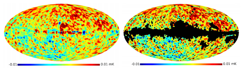
The same is not true, however, for WMAP. Of course WMAP only use the one method of removing foreground, but they did provide different maps based on the data they had collected after 7 years of operation and after 9 years. The ILC9–ILC7 difference map looks quite different:

ILC9–ILC7 difference map on the left, and with a galactic mask overlaid on the right. Figure from arXiv:1305.4033.

Most of the difference appears well away from the galactic plane, as you can see in the right-hand figure, where the galaxy is masked out. So there is some important source of noise that is not foregrounds – so probably some systematics – that has affected the WMAP ILC map. Even more importantly, it is some kind of systematic effect that has changed between the 7-year and the 9-year WMAP data releases, meaning that the ILC9 and ILC7 maps do not appear to be consistent with each other. Frejsel et al. discuss a method of quantifying this, but I won't go into that here because the impression created by the images is both dramatic enough and entirely in line with the quantitative analysis.

As you might have expected, the same method shows that WMAP's ILC9 map is thoroughly inconsistent with the various Planck maps (the picture here is even worse than that between the two ILC maps). But perhaps surprisingly, ILC7 is perfectly consistent with Planck. So it appears that whatever might have affected the WMAP results only affected the final data release.

I guess one should be careful not to make too much of a fuss about this. The results from Planck and WMAP are, generally speaking, in pretty good agreement, except for some problems at the very largest scales. It is also true that the WMAP team themselves do not use the ILC map for most of their analysis (except for the low multipoles, $\ell<32$ – that is, the very largest scales!). But I'm sure this paper will provoke some head-scratching among the WMAP team as they try to figure out what has happened here. Oh, and if you are cosmologist using the ILC9 map for your own analysis, you should probably check whatever conclusions you draw using some other maps before publishing!

All in all, I think I'm rather looking forward to Planck's consistency paper when it does finally come out!

One year on

It has been a long month-and-a-bit since I last had the time to write a proper post here. Primarily this is because I am not very good at doing more than one thing at a time – at least while attempting to do those things properly – and I have been working on some real research papers, which I thought I should try to do properly. As a result science communication, and blogging in general, has had to wait. But I will get back in the swing of things very soon: there are some interesting new results, some interesting rehashes of old arguments about inflation, and one of my own papers that I will write about over the next couple of weeks.

One of the many things that I omitted to mention during this little break was the fact that Blank On The Map had its first anniversary a couple of weeks ago. All in all, I would say it has been quite a satisfying year of blogging, and, at least relative to my prior expectations, a reasonably successful one too. Blogger doesn't provide me with many detailed statistics, but it does tell me that despite the low recent rate of new postings, there have been roughly 23,000 clicks over the last twelve months. A sizeable portion of of this traffic came from one link on Peter Woit's blog (boy he must have a huge number of readers!) – though the majority appear to arrive via Google search, either by accident or design.

Anyway, to all those who have arrived here at some point over the last year, welcome! I hope you found what you were looking for, and enjoyed what you read. This explains what this blog is about. In case you haven't worked your way through the archives, here is a short selection of some highlights from the last year:

• Steven Weinberg and the 'Crisis of Big Science'
• An explanation of a dark matter controversy
• A question of probability
• The dog who climbed a mountain
• The Structure of a Scientific Revolution
• Explaining Planck by analogy

I should also use this post to try to get some feedback from (all three) regular readers. Do you think I should post more often? Less often? More posts about cosmology and fewer about mountaineering and other stuff in general? Or the other way round? Let me know through the comments box. Constructive criticism of the writing style or any other aspect of this blog will also be well received, though I can't promise to change ...