A real puzzle in cosmology: part I

In a previous post, I wrote about recent updates to the evidence from the cosmic microwave background for extra neutrino species. This was something that a lot of people in cosmology were prepared to get excited about, but I argued that reality turned out to be really rather boring. This is because the new data neither showed anything wrong with the current model of what the universe is made of, nor managed to rule out any competing models.

Today I'd like to write about something else, which currently is a really exciting puzzle. Measurements have been made of a particular cosmological effect, known as the integrated Sachs-Wolfe or ISW effect, and the data show a measured value that is five times larger than it should be if our understanding of gravitational physics, our model of the universe, and our analysis of the experimental method are correct. No one yet knows why this should be so. The point of this post is to try to explain what is going on, and to speculate on how we might hope to solve the puzzle. It has been written in a conversational format with the lay reader in mind, but there should be some useful information even for experts.

Before beginning, I should point out that this what a lot of my own research is about at the moment. In fact, this was the topic of a seminar I gave at the University of Helsinki last week (and much of this post is taken from the seminar). My host in Helsinki, Shaun Hotchkiss, with whom I have written two papers on this "ISW mystery", has also put up several posts about it at The Trenches of Discovery blog over the last year (see here for parts I, II, III, IV, V, and VI). I will be more concise and limit myself to just two!

Obviously you could view this as a bit of an effort at self-publicity. But at a time when, both in particle physics and cosmology, many experiments are disappointingly failing to provide much guidance on new directions for theorists to follow, this is one of the few results that could do so. (Unlike a lot of the rubbish you might read in other popular science reports, it also has a pretty good chance of being true.) So I won't apologise for it!

What is the integrated Sachs-Wolfe effect?

The entire universe is filled with very cold photons. These photons weren't always very cold; on the contrary, they are leftovers from the time soon after the Big Bang when the universe was still very young and very small and very hot, so hot that all the protons and electrons (and a few helium nuclei) formed a single hot plasma, the photons and electrons bouncing off each so often that they all had the same temperature. And as the universe was expanding, this plasma was also cooling, until suddenly it was cool enough for the electrons and protons to come together to form hydrogen atoms, without immediately getting swept apart again. And when this happened, the photons stopped bouncing off the electrons, and instead just continued travelling straight through space minding their own business, cooling as the universe continued to expand. (The neutrinos, which only interact weakly with other stuff, had stopped bouncing and started minding their own business some time before this.)

What I've just told you is a cartoon picture of the history of the early universe. These cooling photons streaming through space form the cosmic microwave background radiation, or CMB for short. They fill the universe, and they arrive at Earth from all directions – they even make up about 1% of the 'snow' you see on an (old-school) untuned TV set. 

The most important property of the CMB photons is that, to a very great degree of accuracy, they are all at the same temperature, whichever direction they come from. This is how we know that the universe used to be very hot, and how we learned that it has been expanding since then. It is also why we think it is probably very uniform. The second important property of CMB photons is that they are not all at the same temperature – by looking carefully enough with an extremely sensitive instrument, we can see tiny anisotropies in temperature across the sky. These differences in temperature are the signs of the very small inhomogeneities in the early matter-radiation plasma which are responsible for all the structure we see around us in the night sky today. When the photons decoupled from the primordial plasma, they kept the traces of the tiny inhomogeneities as they streamed across the universe. The matter, on the other hand, was subject to gravity, which took the small initial lumpiness and over billions of years caused it to become bigger and lumpier, forming stars, galaxies, clusters of galaxies and vast clusters of clusters.

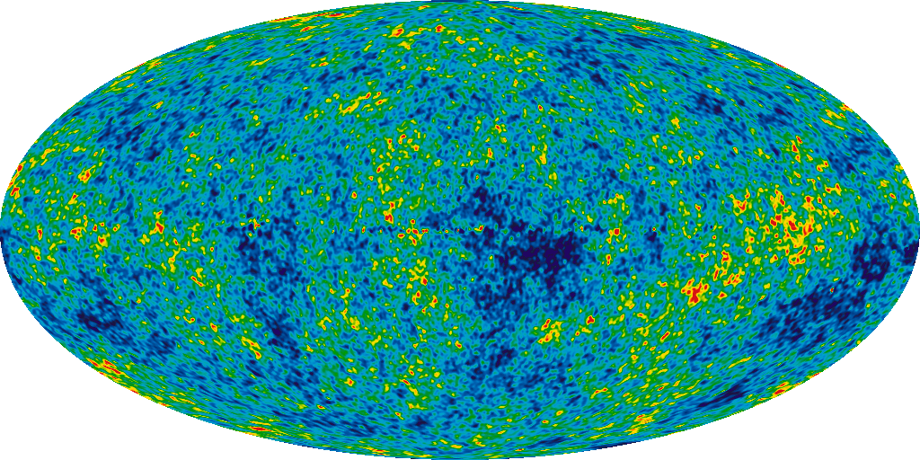The CMB sky as seen by the WMAP satellite. The colours represent deviations of the measured CMB temperature from the mean value – the CMB anisotropies (red is hot and blue is cold). This map uses the Mollweide projection to display a sphere in two dimensions. Image credit: NASA / WMAP Science team. 

Yes I knew that, but what is the integrated Sachs-Wolfe effect?

I'm coming to that. As I said, the CMB anisotropies are largely an imprint of the primordial inhomogeneities in the photon-baryon plasma. But there are also secondary anisotropies, which get added to it at a later stage. The integrated Sachs-Wolfe effect (I'm just going to call it the ISW from now on) is one of these. On their journey through the universe, the CMB photons traverse through the growing lumpiness of matter: clumpy overdense regions and empty void regions. This clumpiness manifests itself as fluctuations in the gravitational potential, $\Phi$. As we know from General Relativity, gravitational potentials affect light. Photons falling in to potential wells gain energy, which they then lose when they climb out the potential hill on the other side.

Except that if the potential $\Phi$ changes with time, the well the photons fall into has a different depth to the hill they later climb up at the other end. This leaves a net change in the energy (and thus temperature) of a photon performing this manoeuvre, which is different in different parts of the sky, adding a secondary anisotropy known as the ISW effect.

A graphical depiction of what I just said. Taken from this webpage.

Why is the ISW effect interesting?

Well, the ISW effect only exists if the potential fluctuation $\Phi$ changes with time. It is only observable if that change is large enough. For a special class of models that we think describe the universe – those with an FRW metric and zero spatial curvature – this means that the ISW effect is observable if and only if dark energy exists. If there is no dark energy, the time derivative of the potential, $\dot{\Phi}$, differs from zero only at second order and the effect is too small to be seen. On the other hand, the existence of dark energy amplifies the effect. You could think of this as being because dark energy accelerates the expansion of the universe and therefore dilutes the lumpiness of structures by 'stretching' them out, so that large potential fluctuations become smaller ('decay') with time. 

A schematic depiction of the ISW effect of over- and under-densities. Image credit: Istvan Szapudi.

So if we can measure the ISW effect at all, this is pretty strong evidence for the existence of dark energy (evidence that doesn't depend at all on supernovae data). The details of the measured effect could tell us about the properties of the dark energy, through the precise way in which it 'stretches' structures – assuming we know or can guess the properties of the initial tiny perturbations which are growing under gravity. Alternatively, if we assume the properties of dark energy (possibly from other observations, like the supernovae), the measurement can tell us about the original perturbations set down very soon after the beginning of the universe itself. Which is pretty amazing!

The problem is, the ISW effect is really small, an order of magnitude smaller than the primary anisotropies in the CMB. So it can't be seen directly. The way it can be detected is by using another dataset in addition to the CMB. Since the ISW effect is caused by matter fluctuations acting on the photons, the ISW temperature fluctuations will be correlated with matter fluctuations – along directions on the sky where there is more matter than average the CMB will tend to be hotter than average because of the ISW shift. So given a large enough catalogue of galaxies which trace the matter distribution, very careful statistical study of the cross-correlation between this and the CMB temperature data can in principle detect the ISW effect.

But it is a tough job. Some attempts at this cross-correlation fail to detect anything, others find positive-but-not-completely-conclusive evidence. And then there is the special puzzling observation.

OK, so what is this puzzling observation?

Back in 2008, a group of scientists in Hawai'i led by Istvan Szapudi decided to look for the ISW effect in a different way. Instead of doing the normal cross-correlation, which uses all the information about all the perturbations however small, they decided to look only at the effects on the CMB of biggest matter density fluctuations.

Naïvely, this might make some sense. The bigger the density fluctuation, the bigger the ISW effect, so in effect by not bothering with all directions they were focussing on only those places where they were expecting the biggest contribution to the signal. However, we know – both because our simplest theory says so and because various other observations confirm – that the distribution of density fluctuations is close to Gaussian. That is, it approximates a bell curve, so that the biggest fluctuations are also the rarest. So by limiting yourself to only the regions that produce the biggest signal, you are in effect throwing away most of the data and limiting your detection power.

No matter. They did the observation anyway. Their method was to use a catalogue of Luminous Red Galaxies (LRGs) created by the Sloan Digital Sky Survey (SDSS) in which a clever computer algorithm helped them identify the positions of overdense and underdense regions. (For experts, it was the Mega-Z photometric LRG catalogue from DR4, with some added area from DR6.) They roughly ranked these regions according to how unlikely they were to have been mistakenly identified, and then selected only the 50 most "significant" of each type. They called these "superclusters" and "supervoids", but in reality the regions were much bigger, and consequently much gentler, fluctuations than those that are normally referred to as "clusters" and "voids" in other contexts.

Then they looked at the CMB along those identified directions and took an average. What they saw looked like this:

Stacked images of the CMB sky along directions associated with "supervoids" and "superclusters" in the SDSS MegaZ LRG galaxy catalogue. The third panel is formed by adding the second panel to the inversion of the first and averaging. Image taken from arXiv:0805.3695.

That looks pretty good! Supervoid directions are cold on average, and supercluster directions are hot. To quantify the evidence, they applied a special filter (a circular compensated top-hat) to the images to reduce the noise and extracted a single number $\Delta T_{\rm avg}$ representing the average temperature shift for these superstructures: the value they got was $$\Delta T_{\rm avg}=9.6\pm2.2\;\mu{\rm K}$$ ($1\;\mu$K is $10^{-6}$ Kelvin, a very small temperature fluctuation indeed!). The error value represents what they got from taking the average temperature along the same number of random directions on the sky, without first identifying any superstructures – this is the noise due to the primary anisotropies on the CMB, which is uncorrelated with structures in the galaxy catalogue. This result was published in the Letters section of the Astrophysical Journal.

What this measured average and error means is that the observed value is roughly $4.4$ standard deviations away from zero. So, barring contamination by some unknown systematic error, the probability that such a value could arise simply by chance (the probability of a false positive detection), is less than $0.1\%$, or odds of roughly $1$ in $16,000$. By cosmological standards, that is rather conclusive evidence of a correlation between the superstructures and CMB temperature fluctuations. 

Well, all this sounds rather good. What's so puzzling about it?

The problem is, the measured value is at least five times too large. Given what we currently know about the universe, the method the Hawai'ian group used should not in fact have been sensitive enough to see any effect at all: the average temperature we would expect to see should at most be only as big as the error bar on the observation due to noise from the primary anisotropies in the CMB. We do not expect such a measurement to give a value significantly far away from zero.

This calculation was made in a wonderful paper written by some great researchers (ok, ok, I was one of the authors) and published last year.

You're going to have to explain that in more detail. How exactly did you calculate what we should expect to see?

I'm glad you asked.

The starting point for the calculation was the fact that, as I mentioned, the matter density fluctuation at any point in the universe is a random variable, with a probability distribution function that is nearly Gaussian. Gaussian random variables are nice and easy to do statistics with. So if you know that the density fluctuation is Gaussian, you can work out the probability of getting a fluctuation of a certain magnitude within a certain region of the universe, or the number of fluctuations of greater than any particular magnitude that should have been present in the MegaZ survey that the observers used. What's more, if a certain point in space has a fluctuation of a certain magnitude, you can also calculate the expected density at nearby points, thus getting the profile of the structure and its total size.

So from this point on we did what physicists normally do: we made a simple model. We assumed the structures seen in the MegaZ survey were due to spherically symmetric structures in the total matter density. Obviously this isn't true for any individual structure, but enough non-spherical structures will – if they are oriented randomly with respect to us – have on average the same effect as a bunch of spherical structures. So we calculated the ISW effect caused by spherically symmetric density fluctuations of various magnitudes and sizes. To do this we assumed the most common model of dark energy, a cosmological constant.

Then we took our calculation for how frequently fluctuations of a given magnitude and size should appear, and weighted our ISW calculation to get the average effect for the $N$ structures that produce the largest ISW effect. Bigger fluctuations (both in spatial extent and magnitude) naturally produce a bigger ISW effect, but as they are further into the tails of the Bell curve they are also rarer and so contribute less to the weighted average. We then used the same filtering technique as in the actual observation, and chose the same number of structures as in the actual observation and found the theoretically expected value for the observation was $$\langle\Delta T_{\rm avg}\rangle\leq2\;\mu{\rm K}.$$ In fact the estimate of $2\;\mu$K – which is still too small to be observed given the background noise – required making all sorts of favourable assumptions and giving the benefit of the doubt to the experiment at every stage, so it was probably an overestimate. Even this overestimate is five times smaller than seen in the measurement. The real value would probably be smaller still.

But I can think of lots of objections to that! What about ...

That's great! We encourage skepticism. But this post is already overlong, so hang on to those objections and we'll discuss them in the next instalment!